The finance question behind the prediction
In cash management and corporate accounting, I learned that finance rarely gets to wait for perfect information. Daily cash positions, funding requirements, loan draws, reporting deadlines, and liquidity decisions depend on information that arrives from different systems at different times. The numbers must reconcile, but that is only the beginning. Finance must also understand what changed, what remains uncertain, and what actions the available evidence supports.
I brought that perspective into Week 5 of the AI for Business & Finance Certificate Program at Columbia Business School Executive Education. The program examines artificial intelligence (AI) through business and finance applications. In Week 5, we moved from linear and logistic regression to decision trees, random forests, model interpretation, and mortgage-prepayment forecasting. My central takeaway was the responsibility an organization accepts when a more accurate model is also more difficult to explain.
This week's material felt familiar because it took me back to my days at San Francisco State University, where I majored in economics and studied econometrics. I learned to use data and statistical models to examine how economic relationships play out in the real world, and my first job in the United States, as an economic analyst at the university, built on that foundation. The mortgage-prepayment case brought many of those ideas back: interest rates, borrower incentives, housing values, and broader economic conditions interacting inside a model. This time, however, I was viewing them through years of experience in accounting and finance. The question was no longer only whether a model could explain or predict behavior. I also wanted to know whether the information would be available in time, whether the results could be supported and reconciled, and whether finance and leadership could responsibly rely on them.
Although random forests were new to me, the decision problem was familiar. A model may improve a forecast, but the people expected to rely on it still have to decide whether the improvement is meaningful, whether the inputs were available when the forecast was prepared, and whether the result can responsibly support a funding or liquidity decision.
That tension is what made the random-forest lesson so interesting to me. I watched a decision tree become increasingly detailed. At first, each additional branch captured a relationship the simpler model had missed. Eventually, the tree became exceptionally good at describing the data it had already seen and less dependable on new observations.
The proposed solution was new to me: build many trees from different samples of the training data and combine their predictions. For a numerical outcome, the forest averages the predictions. For a classification problem, it combines their votes or estimated probabilities. Because the final prediction no longer rests on one tree, the forest can be less sensitive to any single fitted path through the data.
I liked the logic immediately and saw the tradeoff just as quickly. A forest may produce a stronger forecast while making its reasoning more difficult to inspect. For accounting and finance professionals, the choice to rely on that complexity becomes a governance and internal-control decision.
Python was the analytical workbench
During Week 5, we performed the analysis in Jupyter notebooks using Python. The notebooks required us to work through the models rather than receive finished results from a dashboard. Python brought together the underlying business data, the statistical and predictive models, the evaluation measures, and the visualizations in one reproducible workflow. This was classical predictive modeling, not a large language model exercise.
Each function corresponded to a distinct part of the analysis. We loaded, organized, aligned, and transformed the data before training a model. We then fitted the models on one set of observations, evaluated them on observations they had not used for fitting, and inspected what drove their performance.
| Workflow step | Python tools and functions | What the work accomplished |
|---|---|---|
| Prepare the data | pandas read_csv(), merge(), groupby(), pivot(), and shift(); NumPy | Loaded source files, combined datasets, summarized populations, and created time-lagged variables such as prior-period prepayment behavior. |
| Separate the evidence | scikit-learn train_test_split(); time-aware training, validation, and test periods | Kept model fitting and tuning separate from the observations used to evaluate performance on new cases. |
| Fit and apply models | statsmodels ols(); scikit-learn DecisionTreeRegressor, RandomForestRegressor, RandomForestClassifier, fit(), and predict() | Built regression baselines and tree-based alternatives, trained them on historical observations, and generated predictions for held-out data. |
| Measure performance | r2_score(), roc_auc_score(), mean_squared_error(), and mean_absolute_error() | Compared models using measures appropriate to continuous forecasts and classification rankings. |
| Inspect and visualize | permutation_importance(), PartialDependenceDisplay. from_estimator(), Matplotlib, and Seaborn | Examined which variables the fitted model relied on and visualized nonlinear relationships, prediction errors, and performance comparisons. |
Working through the full Python workflow changed how I understood the models. A performance score was no longer an isolated answer. It reflected a chain of choices about data definitions, timing, model settings, comparison metrics, and visual interpretation. For accounting and finance professionals, the practical value lies in understanding each stage well enough to challenge the evidence, reproduce the analysis when necessary, and connect the output to a financial decision.
Why one straight line was not enough
The Week 5 apartment-price exercise made the limits of a single linear relationship easy to see. A linear model begins with a powerful simplifying assumption: the relationship between a predictor and the outcome can be represented by a constant slope unless the analyst deliberately adds transformations or interaction terms.
The class data did not follow that pattern. Price per square foot did not change with apartment size at a constant rate across the full range. The relationship also differed depending on whether the building had a door attendant. A single coefficient on square footage could not represent a relationship whose shape changed or depended on another characteristic.
A decision tree approached the same problem as a sequence of questions. Each apartment followed one branch or another based on characteristics such as building services, size, rooms, floor, and location. That structure could represent thresholds and interactions without requiring one straight-line effect everywhere.
In finance, one input can have a different effect under different circumstances. Customer collections may behave differently depending on the age of a receivable, dispute status, concentration, or the customer's prior payment pattern. A funding need may change sharply around payroll, debt service, a loan-draw deadline, or a minimum cash requirement. These examples do not establish that a tree-based model is appropriate. They show why finance professionals should test whether a single, constant relationship adequately represents operating reality.
That flexibility creates another problem. A shallow tree may miss meaningful distinctions, while a very deep tree may divide observations until it captures peculiarities that will not recur. The appropriate depth must therefore be tested on observations the model did not use for fitting.
This was one of my first aha moments of the week. A deeper tree was not automatically better or worse. Additional branches could capture relationships that mattered, but after a certain point they could also capture noise that belonged only to the training sample. What mattered was whether the added complexity improved predictions for observations the model had never seen.
For cash forecasting, that distinction has practical consequences. A model can reproduce the last reporting period perfectly and still fail when customer behavior changes, a large disbursement moves, or an unusual funding event occurs. Historical fit can support the analysis, but treasury cannot fund the business with a model that only remembers the past.
How random forests reduce reliance on one tree
A random forest manages complexity by fitting many trees to different samples of the training data and combining their predictions. A recurring relationship can appear across multiple trees, while sample-specific noise is more likely to vary from one tree to another.
Because random forests were new to me, I first saw this as a solution to the shallow-tree-versus-deep-tree problem. The more careful lesson was narrower. Combining different trees can reduce the instability and overfitting risk created by relying on one tree, but it does not eliminate either problem.
A forest can still fail for familiar reasons. The data may be poorly defined, information about a future outcome may leak into the predictors, or the training population may differ from the population that will encounter the model. Tree depth and other settings must therefore be tuned without repeatedly testing choices against the final test set.
The full workflow therefore matters. Training data are used to fit the model, validation data help choose the settings, and a separate test set evaluates the final choice. If the same observations are reused across those steps, both the model and the analysts tuning it can adapt to quirks in a single dataset. The resulting score may reflect familiarity rather than performance on new cases. A final test set protects the evaluation because it plays no role in fitting or tuning.
From a control perspective, finance should be able to document which data trained the model, which data influenced tuning, which observations were reserved for final evaluation, and who approved those choices. That record serves a purpose similar to the support retained for a reconciliation or the assumptions behind a cash forecast. Although the calculation may be automated, responsibility for the evidence remains with people.
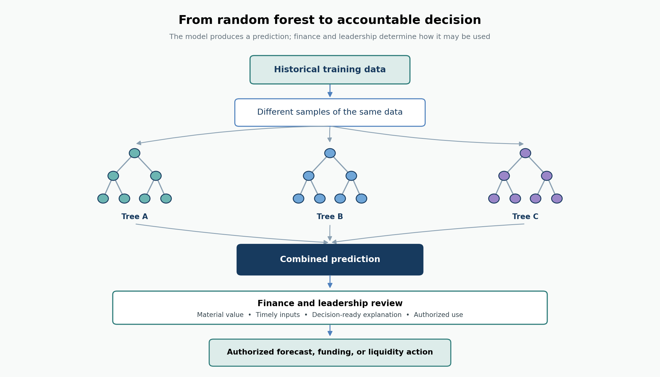
| Step | Figure logic |
|---|---|
| 1 | Historical data is prepared and sampled into multiple analytical views. |
| 2 | Separate decision trees learn different relationships from those samples. |
| 3 | Their predictions are combined into a random-forest prediction. |
| 4 | Finance and leadership review whether the improvement is material, the inputs were timely, the result can be explained, and the proposed use is authorized. |
| 5 | Only after that review may the output support a forecast, funding, or liquidity action. |
The improvement must justify the added complexity
The apartment exercise kept me from treating the random forest as an automatic upgrade. In the classroom comparison, the tuned forest and the more fully specified linear regression both produced an out-of-sample R-squared of about 0.44. R-squared describes how much of the variation in the observed outcome is accounted for by the model. The forest's result was slightly higher, but the difference was very small.
Such a small statistical gain matters only if it changes an operating outcome. Finance should estimate whether the improvement would materially reduce forecast error or prevent avoidable borrowing, idle cash, a delayed loan draw, or a missed funding requirement. The team should also consider how often the model will run and the dollar effect of being wrong. A small improvement may not justify the added development, validation, documentation, monitoring, and explanation. That conclusion could change when the model influences many high-value decisions or when a modest forecast error creates a significant liquidity cost.
The creditworthiness exercise produced a clearer tradeoff. A logistic regression reported an out-of-sample area under the receiver operating characteristic curve (AUC) of 0.68. A tuned random forest reached an AUC of approximately 0.735. AUC measures how well the model ranks higher-risk cases above lower-risk cases across possible classification thresholds; it is not the percentage of applications classified correctly. In the course interpretation, an AUC of 0.68 meant that when comparing one loan that defaulted with one that did not, the model had a 68% chance of assigning the higher risk score to the defaulted loan. The improvement was meaningful within the exercise, but the more complex model was harder to interpret.
That comparison is where my financial-reporting and internal-control experience becomes relevant. Statistical measures show how the models compare. Finance must decide whether the difference changes cash, risk, or decisions enough to justify the implementation and control costs. A better score alone cannot answer that question.
Better prediction can reduce direct explainability
A regression coefficient can often be explained directly, subject to the assumptions and limits of the model. A small decision tree can be followed from its first question to a terminal prediction. A forest containing many trees offers no comparable single path because its final result is assembled from numerous routes through the data.
The course introduced two inspection methods that provide partial visibility. Permutation importance asks what happens to predictive performance when one variable is shuffled and therefore made uninformative. A large decline suggests that the fitted model relied heavily on that variable. Partial dependence shows how the model's prediction changes with a selected variable after averaging over the others.
These methods offer useful but partial explanations. Variable importance does not reveal the direction of a relationship or prove that a variable causes the outcome. Partial dependence describes the model's average behavior; it does not explain every individual prediction or establish that the observed pattern is appropriate to use.
Explanation has practical value in cash forecasting. If a model predicts a shortfall, treasury needs enough context to evaluate the response. Is the change associated with slower collections, a concentration of scheduled payments, a delayed transfer, a large funding requirement, or another factor? A prediction can be statistically useful yet operationally weak if it does not lead to an investigation or action.
My instinct here comes from reconciliations and financial reporting. A reconciliation can tie out mathematically and still contain unsupported items, incorrect mappings, or timing differences that no one has resolved. Likewise, a model can outperform a baseline and still lack the support finance needs before relying on its conclusion.
The loan exercise revealed another limitation. The historical dataset contained completed loans, so every borrower in it had already passed an earlier approval process. The model could observe default outcomes only among borrowers who received credit. It could not tell us how rejected applicants would have performed. The training population therefore carried the effects of prior business decisions into the new model.
As a Certified Public Accountant, I see interpretability as a practical requirement. The level required depends on how the model will be used. A model used for exploratory analysis, risk-based pricing, a human recommendation, or an automated credit decision creates different needs for explanation, challenge, approval, and documentation.
A forecast becomes useful when finance can connect the prediction to evidence, an action, and an accountable decision owner.
The mortgage case made cash flow uncertainty visible
The mortgage-prepayment case brought these questions together in one financial system. A borrower with a 30-year fixed-rate mortgage makes a constant scheduled payment, but the composition changes over time. Interest is highest early because the unpaid balance is highest. Scheduled principal gradually becomes a larger share as the balance declines.
The classroom amortization example gave me a more personal reaction than I expected. For a $400,000, 30-year mortgage at the illustrated 7% rate, the total scheduled interest over the life of the loan exceeded the original principal. A monthly payment that appeared manageable could conceal a much larger lifetime financing cost. That realization made refinancing and prepayment feel far less abstract.
Borrowers can also repay principal earlier than scheduled, often because they refinance or sell the home. That can benefit the borrower, but it changes the timing of cash flows expected by an investor in a mortgage-backed security. The borrower's opportunity to refinance becomes the investor's prepayment risk.
That was another aha moment for me. The same refinancing decision can reduce a borrower's future interest while disrupting an investor's expected cash flows. I began to see the case primarily as a cash-flow forecasting problem. The contractual schedule alone does not determine the cash-flow schedule because people can act. The forecast must therefore account for behavior, timing, and changing economic incentives. A technically stronger model matters only if it improves the organization's ability to anticipate those cash flows and manage the consequences.
The model did not predict whether one named borrower would refinance. Its unit of analysis was a mortgage pool in a particular month. Pools were organized by origination period and coupon range. The target was the following month's conditional prepayment rate (CPR), which annualizes the monthly share of the pool's outstanding mortgage balance that prepays.
The inputs represented different parts of the economic story. They included recent prepayment behavior and the difference between the pool's existing mortgage rate and the rate available on a new mortgage. The dataset also included loan-to-value, debt-to-income, credit, pool age, unpaid balance, estimated home equity, transaction mix, geography, seasonality, home prices, and broader economic conditions.
The rate incentive was especially intuitive. When the existing mortgage rate is higher than the current market rate, refinancing becomes more attractive. Yet the relationship with prepayment was not a straight line. It was relatively flat when refinancing offered little benefit, increased as the incentive became favorable, and flattened again after many of the borrowers most responsive to refinancing had already left the pool. The remaining population had changed. The course described this as burnout.
That pattern explained why a tree-based model could add value. The effect of one variable could change across ranges and interact with the history and composition of the pool. The forest could capture those thresholds without requiring the analyst to specify every possible nonlinear term in advance.
The same discipline applies when finance evaluates a cash or liquidity model. The economic meaning of each variable matters. A balance, aging bucket, scheduled payment, draw request, or customer-history field is not useful merely because it is available in a dataset. Finance must understand why it could affect cash, how it was measured, and whether the relationship remains plausible when business conditions change.
The strongest predictor arrived too late
The mortgage results delivered the week's most practical lesson. In the Python notebook, we compared each model's predicted conditional prepayment rate with the actual rate in out-of-sample testing data. One reported measure was root mean squared error (RMSE), which summarizes the size of prediction errors; a lower RMSE indicates smaller errors. The random forest with a maximum depth of four produced the lowest reported RMSE among the models tested. It therefore performed best on that measure in the classroom comparison, but that did not make it automatically the best model to use in practice.
To understand why, the class used permutation importance. Conditional prepayment rate (CPR) from the preceding month was the strongest predictor, followed by CPR from two months earlier and the recent refinancing incentive. In modeling language, those earlier values are described as lagged CPR.
An operating constraint then changed the analysis. The mortgage-performance data needed to calculate recent CPR and unpaid balance could arrive with a delay of roughly five to six months. A database might eventually contain those observations, but a forecaster trying to predict next month's prepayment rate would not yet have them.
The class rebuilt the model without the unavailable recent information. Under that constraint, the reported RMSE increased from 12.3% to 12.9%, mean absolute error (MAE) increased from 7.5% to 8.6%, and the constrained model's R-squared was 25.7%. RMSE gives greater weight to larger misses, while MAE reports the average absolute size of the error. R-squared describes how much variation in the outcome the model accounts for.
Although the scores were weaker, the constrained test answered the operational question more honestly. The unconstrained model estimated what could be predicted with information that would eventually exist. The constrained model estimated what could be predicted with information available at the forecast date.
This was my strongest aha moment in the mortgage case. Information may eventually appear in a database and still be unavailable when today's decision must be made. Predictive strength and operational usefulness are not the same thing.
That distinction is familiar from accounting and cash management. Evidence has an as-of date. In practice, bank activity, subsidiary reporting, invoices, payment information, and funding requests may become visible on different schedules. A later value can sharpen hindsight without improving the forecast that finance actually had to prepare. If the production process cannot obtain an input by the cutoff, historical access to that input does not make the forecast deployable.
This is also an internal-control issue. The organization should define the forecast cutoff, document which sources are expected by that time, identify estimates or substitutions, and retain evidence that the model used the version of the information available then. Without that discipline, the reported test may overstate what finance could have known.
A model evaluated with information that arrives too late measures hindsight rather than the forecast finance could actually produce.
What I would require before the organization relies on the model
The three cases gave me a practical standard for evaluating complexity. Before a predictive model influences a cash forecast, funding plan, or liquidity decision, I would expect the case for relying on it to address five areas.
- The financial decision. What exactly is being forecast, for what period, and at what level of detail? How will the prediction change a cash, funding, or liquidity decision, and who is authorized to act on it?
- Value of the improvement and cost of error. How much does the model improve on an appropriate simpler baseline when both are evaluated on unseen data? What is the dollar consequence of the remaining error, and is the improvement large enough to justify the added cost and control burden?
- Input timing and traceability. Were all predictors available by the forecast cutoff? Can finance trace each important input to its source, definition, transformation, and as-of date, and can the model input be reconciled to the underlying operational or financial record?
- Population relevance. Which customers, transactions, properties, or reporting periods appear in the training data, and which are absent because of earlier decisions or unusual conditions? How closely does that population resemble the activity finance expects the model to forecast?
- Explanation, accountability, and monitoring. Can the result be explained at the level required for the decision? Who reviews exceptions, approves overrides, compares forecasts with actual cash results, and determines when deterioration requires recalibration or suspension?
These questions do not yield a universal threshold for complexity. A modest improvement may be valuable in a high-volume process with costly forecast errors and strong controls. A larger gain may still be unacceptable if it depends on information finance cannot obtain on time, a population that does not match current activity, or an explanation that does not support the decision.
What finance and leadership must own together
The technical work in these cases was sophisticated, but the decision to rely on a model cannot rest only with its builders. Finance should help define the economic outcome, forecast horizon, information cutoff, and financial consequences of prediction errors.
Leadership and the designated decision owners must determine what level of error is acceptable, authorize how the model's output may be used, and remain accountable for the actions that follow. When the model affects processes outside finance, the people responsible for those operations must also participate.
Model builders remain responsible for explaining how the data was assembled, how the model was tested, and what its limitations are. Finance must be able to challenge the analysis and translate its implications into business consequences. Leadership need not reproduce the technical work, but it must understand what could happen if the prediction is wrong before authorizing reliance on it.
My work in cash management, funding, loan draws, reporting, reconciliations, and internal controls shapes this view. In those settings, a number is useful when it can be traced to evidence, placed in the correct period, reconciled where appropriate, explained to the people responsible for acting, and reviewed against actual results. A predictive output should not be held to a lower standard merely because its calculation is more sophisticated.
Accounting and finance professionals are trained to test definitions, populations, cutoffs, reconciliations, assumptions, and evidence while evaluating materiality and responsibility. That training does not make us data scientists or model validators. It does prepare us to determine whether a model's reported performance supports the financial decision the organization intends to make.
This shared responsibility requires professional humility. Permutation importance can identify variables the model depends on, but it cannot determine whether those variables are appropriate. A partial dependence plot can reveal an unexpected threshold, but it cannot explain the business reason without further investigation. A strong test score can provide predictive evidence within the sample while leaving questions about deployment, fairness, economics, and changing conditions.
I want enough command of the modeling process to ask credible questions about the data, tuning, performance measures, the visibility lost as complexity increases, and the conditions required before the output can support a finance decision.
The standard I will carry into practice
The course left me with a set of questions that finance and model-building teams should answer together. How should a reduction in forecast error be translated into liquidity value? What explanation does treasury need before acting on an ensemble prediction? How should the team document model inputs and cutoffs alongside existing forecasting controls? When is the strongest historical predictor too delayed to be useful in production?
The three cases answered those questions differently. In the apartment example, the forest added very little predictive value. In the creditworthiness example, it improved performance more meaningfully. In the mortgage case, the relevant benchmark was the performance achievable with information available under the timing constraints of the real process.
Before relying on a complex model, I want to know what measurable value it adds, which information it requires at the decision date, and what explanation and controls the decision demands. Finance must be able to reconcile the inputs and explain the financial consequences. Authorized leaders must understand the risk and remain accountable for the action. If those conditions are not met, a higher test score is not enough.
A more accurate model earns organizational reliance only when its improvement is material, its information is timely, and its output supports an accountable decision.
The Model Reliance Framework
This framework helps finance, accounting, leadership, and model teams evaluate whether a model's reported improvement is ready to influence a consequential decision. It separates predictive performance from organizational authorization. A higher score begins the review; it does not end it.
The five reliance questions
Financial decision
What decision changes, and who may act?
Material value
Is the improvement worth the remaining error and added control cost?
Timely evidence
Were the inputs available at the decision cutoff?
Relevant population
Does the historical population support the intended use?
Explanation and accountability
Can the result be challenged, approved, and monitored?
CPA Insight
A more accurate model earns organizational reliance only when its improvement is material, its information is timely, and its output supports an accountable decision.
Companion Practical Resource
Practice Guide No. 005 - The Predictive Model Reliance Review is a structured review for evaluating value, timing, population, explanation, accountability, and monitoring before a predictive model influences a consequential decision.
Sources and learning note
This article reflects my personal interpretation of concepts studied in the advanced predictive analytics portion of the AI for Business & Finance Certificate Program offered by Columbia Business School Executive Education. It is an independent reflection and does not imply endorsement by Columbia Business School, its faculty, or the program's collaborators.
The classroom examples discussed are The Zestimate Revisited, Predicting Creditworthiness, and Real Estate Analytics: Mortgage Prepayment Prediction. References to Python libraries and functions identify the workflow; course code, slides, prompts, transcripts, datasets, and proprietary instructional language are not reproduced. The personal reactions, Figure 1, and finance applications are my own interpretations.
Disclaimer
This article is educational and does not provide investment, lending, accounting, legal, or model-risk advice. Organizations should involve qualified professionals and evaluate applicable requirements before using predictive systems in consequential decisions.
Related Knowledge Hub materials
This article continues my exploration of how accounting and finance professionals can use emerging technologies while preserving evidence, governance, controls, professional judgment, and accountability.
About the author
Valentina DuPont, CPA is an accounting and finance professional with experience in financial reporting, month-end close, reconciliations, cash management, internal controls, audit support, and process improvement. Through the Knowledge Hub, she explores how professional judgment, governance, and emerging technologies intersect in modern finance.